Fast Fourier Transform
In an algorithms class I took last semester (6.046), we learned about the Fast Fourier Transform (FFT) as an example of a divide-and-conquer algorithm. That was one of my favorite lectures, so I thought I'd write a blog post about the concept.
Motivation
Given two degree-\(n\) polynomials \(A(x)\) and \(B(x)\), how would you compute their product \(C(x) = A(x) \cdot B(x) \)? A naive method would be to multiply each pair of terms in \(A(x)\) and \(B(x)\) and combine resulting terms with equal degree. Because \(A(x)\) and \(B(x)\) each have \(O(n)\) terms, computing \(C(x)\) in this way takes \(O(n^2)\) time. However, using FFT the product can actually be computed in \(O(n\log{n})\) time. That's a pretty dramatic speedup! Let's see how this is accomplished.
Setup
The first idea behind the FFT-method for polynomial multiplication is that polynomials have two representations. The more common one is the coefficient representation, in which we specify the coefficents of each power of \(x\): for example, \(f(x) = 1\cdot x^2 + 0\cdot x - 1 = x^2 - 1\).
In the point-value representation, we instead describe a degree-\(n\) polynomial using \(n+1\) distinct points \((x_k, y_k)\) that the polynomial intersects. This representation is valid because of the fact that two degree-\(n\) polynomials cannot share \(n+1\) identical points[1]. For example, if we choose the points \((-1, 0), (0, -1), (1, 0)\), then \(f(x) = x^2 - 1\) is the unique quadratic that interesects all three. Note that there are infinite other sets of points we could have chosen to represent \(x^2 - 1\), one such set being \((1, 0), (2, 3), (3, 8)\).
The point-value representation is important because polynomial multiplication can be performed in linear time if we only care about the point-value representations of the polynomials. To see why, observe that if \(A(x)\) and \(B(x)\) are degree \(n\), then their product \(C(x)\) is degree \(2n\). Then, assuming we know the values of \(A(x)\) and \(B(x)\) at \(2n+1\) different locations \(x_k\), we can compute the value of \(C\) at each of those points in \(O(n)\) time by iterating over each location and computing \(A(x_k)\cdot B(x_k)\).
To summarize, naively multiplying polynomials in coefficent form requires \(O(n^2)\) time, while multiplying polynomials in point-value form only takes \(O(n)\) time. Since we typically are given the input polynomials in coefficent form, and want the product to be in coefficent form as well, the final step is to figure out how to convert a polynomial between the two forms efficiently. That's where FFT comes in.
Converting between forms using FFT
Given a polynomial \(A(x) = a_0 + a_1\cdot x + \cdots + a_n \cdot x^n\), we want to evaluate it at \(2n + 1\) different points \(x_k\). Using Horner's Method, evaluating a polynomial at one point takes \(O(n)\) time, so in total this would generally take \(O(n^2)\) time.
However, if we choose the values of \(x_k\) carefully, we can reduce the time complexity to \(O(n\log{n})\)! I will first state what these special values are, then I will prove the \(O(n\log{n})\) runtime. (Note: the proof uses complex numbers, specifically roots of unity. If you are unfamiliar with this topic, I recommend watching some of KhanAcademy's videos.)
First, let \(N\) be the smallest power of two that is at least \(2n + 1\). We can treat \(A(x)\) as a degree-\((N - 1)\) polynomial with \(a_i = 0\) for \(n < i < N\). This will make the proof simpler.
The special values that we will evaluate \(A(x)\) at are \(x_k = e^{\frac{2\pi i}{N}k} = \omega^k\), aka the \(N\)-th roots of unity. Because \(N > n\), this set of points uniquely determines \(A(x)\).
To compute \(A(x)\) at each \(N\)-th root of unity, we will use a divide and conquer algorithm. Define the two polynomials \(A_{even}(x) = \sum_{i=0}^{\frac{N}{2} - 1} a_{2i} x^i \) and \(A_{odd}(x) = \sum_{i=0}^{\frac{N}{2} - 1} a_{2i + 1}x^i\). In other words, \(A_{even}(x)\) contains all the even-indexed coefficients of \(A(x)\), and \(A_{odd}(x)\) contains all the odd-indexed ones. Both have degree \(\frac{N}{2} - 1\).
Observe that \[ A(x) = a_0 + a_1 x + \cdots + a_{N - 1} x^{N - 1} \] \[ = (a_0 + a_2 x^2 + \cdots + a_{N - 2} x^{N - 2}) + x(a_1 + a_3 x^2 + \cdots + a_{N - 1} x^{N - 2}) \] \[ = A_{even}(x^2) + xA_{odd}(x^2) \]
Now, the benefit of using roots of unity appears. Because \(x_k\) form the \(N\)-th roots of unity, and because \(N\) is a power of two, the set of values \((x_k)^2\) actually form the \(\frac{N}{2}\)-th roots of unity! This can be shown more rigorously by observing that \((x_k)^2 = (e^{\frac{2\pi i}{N}k})^2 = e^{\frac{2\pi i}{N/2}k} \).
Therefore, to evaluate \(A(x)\) at all \(N\)-th roots of unity, we need to first evaluate \(A_{even}\) and \(A_{odd}\) at the \(\frac{N}{2}\)-th roots of unity, then combine the results. The combining step takes \(O(N)\) because we just iterate over each of the \(N\)-th roots of unity, so if we let \(T(N)\) represent the time complexity of evaluating a degree-\((N - 1)\) polynomial at the \(N\)-th roots of unity, we get the recurrence relation \(T(N) = 2T(\frac{N}{2}) + O(N)\). Applying the master method gives us that \(T(N) = O(N\log{N})\). Because \(N = O(n)\), this means we can evaluate our polynomial at \(2n + 1\) points in \(O(n\log{n})\) time, which is what we originally set out to prove.
We can express this more succinctly using linear algebra: \[ \begin{bmatrix} 1 & 1 & \cdots & 1 \\ 1 & \omega & \cdots & \omega^{N-1} \\ 1 & \omega^2 & \cdots & \omega^{2N - 2} \\ & & \cdots & \\ 1 & \omega^{N - 1} & \cdots & \omega^{(N - 1)^2} \end{bmatrix} \cdot \begin{bmatrix} a_0 \\ a_1 \\ a_2 \\ \cdots \\ a_{N - 1} \end{bmatrix} = \begin{bmatrix} A(x_0) \\ A(x_1) \\ A(x_2) \\ \cdots \\ A(x_{N - 1}) \end{bmatrix} \] FFT gives us a way to perform this matrix multiplication in \(O(N\log{N})\). We can use the same method to compute the point-value form of \(B(x)\) in \(O(n\log{n})\). Finally, we can compute the point-value form of \(C(x)\) in \(O(n)\) as discussed earlier.
Inverse FFT
Once we know the point-value form of \(C(x)\), we can use the inverse FFT to compute its coefficents \(c_i\). Its coefficients satisfy the equation: \[ \begin{bmatrix} 1 & 1 & \cdots & 1 \\ 1 & \omega & \cdots & \omega^{N-1} \\ 1 & \omega^2 & \cdots & \omega^{2N - 2} \\ & & \cdots & \\ 1 & \omega^{N - 1} & \cdots & \omega^{(N - 1)^2} \end{bmatrix} \cdot \begin{bmatrix} c_0 \\ c_1 \\ c_2 \\ \cdots \\ c_{N - 1} \end{bmatrix} = \begin{bmatrix} C(x_0) \\ C(x_1) \\ C(x_2) \\ \cdots \\ C(x_{N - 1}) \end{bmatrix} \] \[ \Longrightarrow \begin{bmatrix} c_0 \\ c_1 \\ c_2 \\ \cdots \\ c_{N - 1} \end{bmatrix} = \begin{bmatrix} 1 & 1 & \cdots & 1 \\ 1 & \omega & \cdots & \omega^{N-1} \\ 1 & \omega^2 & \cdots & \omega^{2N - 2} \\ & & \cdots & \\ 1 & \omega^{N - 1} & \cdots & \omega^{(N - 1)^2} \end{bmatrix}^{-1} \cdot \begin{bmatrix} C(x_0) \\ C(x_1) \\ C(x_2) \\ \cdots \\ C(x_{N - 1}) \end{bmatrix} \] The roots of unity satisfy the property that \(1 + \omega + \cdots + \omega^{N-1} = 0\). This can be used to show that the inverse of the matrix is \[ \frac{1}{N} \cdot \begin{bmatrix} 1 & 1 & \cdots & 1 \\ 1 & \omega^{-1} & \cdots & \omega^{-(N - 1)} \\ 1 & \omega^{-2} & \cdots & \omega^{-(2N - 2)} \\ & & \cdots & \\ 1 & \omega^{-(N - 1)} & \cdots & \omega^{-(N - 1)^2} \end{bmatrix} \] This is almost the same as the matrix equation to convert from coefficient to point-value form, except the exponents have changed sign and there is a factor of \(\frac{1}{N}\). Therefore, we can apply a similar divide-and-conquer algorithm, known as the inverse FFT, to convert \(C(x)\) from point-value form back into coefficient form.
Summary
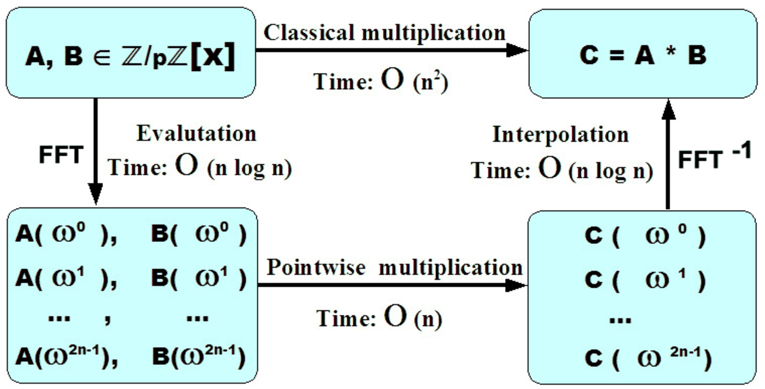 This diagram, from these lecture notes, is a great summary of how FFT speeds up polynomial multiplication.
Acknowledgements
Thanks Rohan Joshi for helping me proofread this post.
Footnotes
- Let \(f\) and \(g\) be two degree-\(n\) polynomials that have \(n+1\) points in common, ie. \(f(x_k) = g(x_k)\) for \(n+1\) different values \(x_k\). Then, the polynomial \(h(x) = f(x) - g(x)\) is equal to zero at each \(x_k\), which means it has at least \(n+1\) roots. However, because \(f\) and \(g\) are degree \(n\), the polynomial \(h\) must also have degree at most \(n\). By the fundamental theoreom of algebra, the only way that \(h\) can have degree at most \(n\) but at least \(n+1\) roots is if \(h(x) = 0\). This implies that \(f = g\), ie \(n+1\) points uniquely defines a degree-\(n\) polynomial. Back to text.